Stitching Microscope Images using Hugin (Free and Open Source)
- Derek Leung

- Mar 7, 2022
- 13 min read
Updated: Mar 9, 2022
If a panorama consists of many pictures,
And each picture is worth a thousand words,
Then the number of words in a panorama must be
Breathtaking.

If you're in the earth sciences, physical sciences, or life sciences, chances are that you're looking at a cool sample under an optical microscope—whether it be a rock, alloy, or tissue—and you want to capture the whole slide in exquisite detail. However, the resolution under the microscope comes at a cost: the field of view shrinks proportionally with higher magnification. To capture a whole slide, it's necessary to photograph individual images, move the sample, and repeat the process. Then, these images have to be stitched into a panorama or tiled mosaic. It's the same principle for large-area images taken with a scanning electron microscope. In this blog post, we'll walk through image stitching of microscope images using Hugin, a free and open-source program.
Why waste time making a tutorial?
Photography fanatics know that there are many programs out there for stitching photos into panoramas. For example, Photoshop, PTGui, and Microsoft ICE are a few programs that come to mind, and they are easy to use. But if you're a thrifty scientist like me, shelling out $30 per month for Photoshop or $200–$400 for PTGui is an unnecessary luxury, especially when there are free alternatives out there. However, it's not just about cost: some programs, such as Photoshop and Microsoft ICE, sacrifice control for ease of use. For my purposes, the quality of the stitching is critical, especially if I want to conduct digital image analysis on the stitched image. This means choosing a program that gives me control over the stitching process, such as PTGui. I am also a huge proponent of the maker movement, which in this case means embracing free and open-source software, but these software can have steep learning curves.
Microsoft's Image Composite Editor (ICE) is a good free (but not open source) program: it has an intuitive user interface where you can drag and drop images, and it has several layout options, such as simple (read: brainless) and structured grid options. I was immediately impressed when I started using Microsoft ICE. However, I quickly ran into problems with Microsoft ICE. The simple layout means that customization is limited, which is mostly a problem when the images don't stitch properly. Moreover, there's a software bug in Microsoft ICE that incorrectly processes vignetting, leading to progressive brightness gradients. Unfortunately, Microsoft ICE is no longer being maintained nor available for download, so those issues will never be fixed.

Fiji/ImageJ is another common tool for processing and analyzing images, which is free and open source. There are several plugins in Fiji/ImageJ that offer image stitching, but I found that they either have bugs, are not optimized for this use, or are too complicated for my simpleton knowledge of clicking buttons and following instructions.
Hugin: An old answer to an old question?
Hugin is arguably the best free and open source software for making panoramas from photos. Like PTGui, it is incredibly powerful, being based on the Panorama Tools library, and it also supports Enblend and Enfuse. These libraries can also be used in the command line, which enables scripting and batch processing. I had known about Hugin for years, but several hurdles prevented me from learning it.
First, its user interface is not as user-friendly as the other software mentioned above. Second, the sheer number of projection methods, camera parameters, and image parameters is confusing when I need everything to be planar! Third, some of the tutorials are about ten years old, so some of the layout has changed since then, and the tutorials can be confusing to follow. There has been some discussion online about using Hugin for grid stitching, but it's not comprehensive. This blog post was inspired by a question on the Photography Stack Exchange and the associated Stitching flat scanned images Hugin tutorial.
Before stitching
Garbage in, garbage out. Remember that image stitching can only be as good as the original images that you take, so carefully consider what images are needed, how these images will be taken, and how they will be processed. It's always best to test a workflow with a small image set before trying more complex scenarios.
For stitching microscope images, consider the following. First, what is the required minimum resolution and mosaic size? Imaging a full slide at 40x objective magnification is probably not realistic (I have a PhD to finish, after all). Second, the images need to have a sufficient overlap (ideally 30–50 % overlap between two images, but lower in some cases) so that the program can identify features or control points to properly align the images. More overlap is generally better, but this means taking even more photos (this is a non-issue if you have an automated stage). Third, the edges of the images are usually worse than the centres because of lens distortion and incongruent lighting. There are ways to correct for these issues (deconvolution microscopy and normalization), but it may be worth using sufficient overlap and/or cropping out the edges to avoid this hassle altogether. Again, test these parameters with a subsample before diving deeper.

Image stitching with Hugin
I'm using Version 2021.0.0.52df0f76c700 of Hugin on a 64-bit version of Windows 10. It defaults to the simple interface on opening. The workflow can be summarized in the following image and steps:

Step 1: Setting up the interface
We'll need to use the expert interface in order to adjust the cumbersome optimization details and lens parameters. (Congrats, you're an expert already! Is the imposter syndrome kicking in yet?) Go to Interface > Expert.
The expert interface has some key features that we'll use:

Photos tab. Image tiles are listed here as a sequence of rows. The Feature Matching and Optimize sections in this tab will be used for producing control points and then aligning the images based on those control points.
Control Points tab. Here, you can view control points and manually add control points.
Show Control Points button. This opens a new window and lists the control points as rows. It is handy for deleting erroneous control points after automatic feature matching or optimization.
Preview Panorama (OpenGL) button. This will be used to review the optimized result and make further corrections, if necessary.
Stitcher tab. We'll use this to produce the final stitched image.
There's also a hidden Optimizer tab that we'll look at later in Step 3.
Step 2: Importing data
Drag and drop the images that will be stitched (alternatively Edit > Add Image...). A new window will pop up asking for Camera and Lens data. For Lens type, select Normal (rectilinear) and for HFOV (v), enter 10. The HFOV, or horizontal field of view, is a camera-specific parameter that differs between telephoto, rectilinear, and fisheye lenses.

The Photos tab in the expert interface looks like this:

Each image is represented by a row, and the rows are in sequence based on the order that they were selected. At this point, it is helpful to choose an anchor for the images, which defaults to the first image. This image will not be shifted during the optimization process. The choice of anchor is not critical (and can be changed at any time), but I usually choose an image in the centre. To set the anchor, select the specified image and right click, then click Anchor this image for position and Anchor this image for exposure. You will see the letters A and C in the Anchor column for that image.
Step 3: Setting optimization parameters
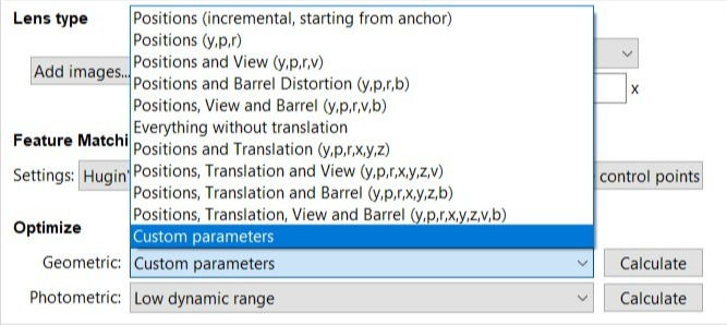
Now, we need to specify the type of motion that is allowed for the image stitching. We need a custom setup because we are translating the camera without rotation, but Hugin is not meant to do this by default. In the Photos tab, go to the Optimize section at the bottom left of the screen. To the right of the Geometric parameter is a dropdown box, where we'll select Custom parameters. Selecting this option allows access to a new tab called the Optimizer.
The Optimizer tab estimates the orientation of the camera when it captured each image. This includes rotation in three directions [up and down (yaw), left and right (pitch), and like a steering wheel (roll)], as well as translation in three directions (X, Y, and Z). Since our microscope setup has a stationary camera, the X and Y parameters should be optimized for all images, whereas the rotational positions and Z should be fixed to 0. At the end of this step, the Optimizer tab should resemble this:

When the microscope images are imported, they are given default rotational positions (you may notice that the Yaw (y) field has a non-zero position). To reset the rotational positions for all of the images, right click on any row in the Image Orientation section and select Manipulate image variables.... A new window will open with some default code.

Paste the code below and press OK. All of the yaw, pitch, and roll values should now be set to 0. (This can also be done manually by right clicking each row and selecting Reset > Reset positions.)
# set yaw to 0
y=0
# set pitch to 0
p=0
# set roll to 0
r=0
To optimize for X and Y only, right-click the Yaw (y) column and click Unselect all. Repeat this for the Pitch (p) and Roll (r) columns. Then right-click the X (TrX) column and click Select all. Repeat for the Y (TrY) column.
In the Lens Parameters section, check Hfov (v). The other parameters a, b, c, d, e, g, t can be left unchecked. These correspond to lens-specific correction parameters and unchecking them makes the assumption that the camera is perfectly rectilinear. These parameters can also be optimized at any time by activating the respective check box.
Step 4: Feature matching
Now, we're ready to add some control points. There are two ways to add control points: automatically and manually. We'll look at both scenarios.
For automatic feature matching, go to the Photos tab and under Feature Matching, press Create control points. The default setting should be Hugin's CPFind. This is fine for image sets with < 40 images. For larger image sets, we'll have to optimize this setup since it takes too long (see Sitching larger image sets section). A log window will pop up and Hugin will iterate through different image pairs to find control points.

If the automatic feature matching doesn't work, then you may need to resort to manual feature matching. Thankfully, Hugin has a good setup for this. The Control Points tab displays two images, and above these images are two dropdown boxes, where different images can be viewed. Select two different images that are neigbouring. Find a spot that is the same between both images. Click that spot in the first image, and then click the spot in the second image. A close-up of the point will appear in both images. Be as accurate as you can be, but by default, Hugin runs auto fine-tune so that the spots match up to one-tenth of a pixel.

When satisfied with the control point, right-click or press Add in the bottom-right corner. This will add the control point and give it an ID number. Ideally, each image pair should have at least three control points, although 1 control point may also work here because we are only optimizing for X and Y (there's no rotation involved). We can always add control points later to improve the stitching. Don't forget to save your project periodically, so that you can take a break and come back to work with fresh eyes.
Step 5: Geometric optimization
Since we set the optimizing parameters in Step 3 so that only translation is allowed, all we have to do to optimize is to click a button. In the Photos tab, under Optimize > Geometric, click Calculate. We can now check how well the images stitched and reassess the optimization. Some of the automatic control points may be false positives, and we need to remove them.
Step 6: Preview
To preview the stitched image, go to Preview Panorama (OpenGL) (also accessed through View > Fast panorama preview window).
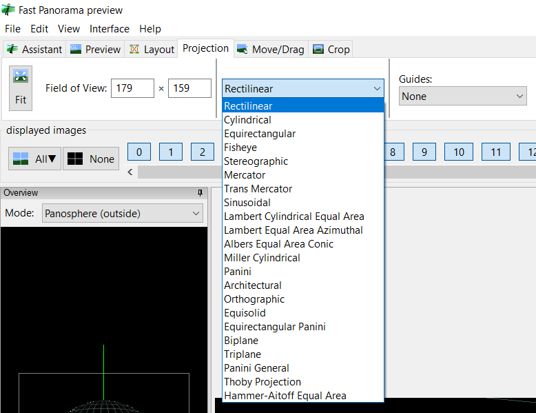
This will open a new window. In the Projection tab, set the projection type to Rectilinear. The weird panosphere overview mode on the left-hand side of the screen can be ignored.
Now, press Fit to hone in on the stitched image. Zoom into the stitched image using the mouse wheel and pan by holding down the mouse wheel and dragging. You can also use the slider bars on the right and bottom to adjust the horizontal and vertical fields of view. Don't worry if the view isn't centred—we can fix this later.
Step 7: Deleting erroneous control points
Sometimes the automatically identified control points are false positives. To see these control points, go to the Preview tab and check Show control points. The control points will show up as x marks in green, yellow, and red, with the colour showing the distance error between the two control points (red is bad).

The easiest way to delete these two control points is by filtering by distance. To do this, go back to the main Hugin - Panorama Stitcher window and click the Show control points button or alternatively, View > Control point table.
A new window will open listing the control points and the distance errors between the control points. Scan through the table to determine the distances of outlier values, but they'll probably have a distance > 10–50. Click Select by Distance at the bottom of the window, which opens another window. A default value for the threshold distance is given. Press OK. This will select the control points with that error or more. Then press Delete to delete those control points. You should see that the erroneous control points have been removed. If not, try a lower threshold value.

Step 8: Troubleshooting missing or problematic tiles
If there are any missing or problematic tiles, you may need to manually add control points for these tiles. To identify these tiles, go to the Fast Panorama preview (OpenGL) window > Preview tab. Activating Identify or holding Ctrl while hovering over the tiles shows the tile number of the image. Images can also be shown or hidden by clicking on the numbers in the displayed images section.

Once you've identified the offending tile(s), it may help to move it to the right area in order to determine its neighbouring tiles. Go to the Move/Drag tab, and select mosaic or mosaic, individual option for Drag Mode. The mosaic mode will move all tiles that are linked by control points, whereas the mosaic, individual mode will move specific tiles (these have to be checked in the displayed images section). You can also use the Layout tab to see how the tiles are related to each other.

Step 9: Repeating Steps 4 to 8
Repeat Steps 4 to 8 to manually add control points, optimize, preview, filter control points, and fix incorrectly stiched tiles. Optionally, you can change the optimization parameters (Step 3) to keep the position of certain tiles fixed. Remember to save your project frequently, especially when the result is improving (the optimization can implode). When you're happy with the layout, continue to the final step: stitching your image!
Step 10: Stitching the final image
Before stitching the image, we can crop the field of view in the Fast Panorama preview (OpenGL) window. Hovering over the preview shows four boxes, which can be dragged to crop the field of view.

When satisfied with the cropping, close the Fast Panorama preview (OpenGL) window and return to the main Hugin - Panorama Stitcher window. Go to the Stitcher tab and check to make sure that the Projection is Rectilinear. For Canvas Size, click Calculate optimal size. This should preserve the resolution of the stitched image. We set the cropping above, so we don't need to change it now. Select the desired output format and compression, and then press Stitch!

A prompt will save the project and ask for the file name of the finished panorama. The Batch Processor will now launch and stitch your image. We're done!
Now that we've successfully stitched our first image, you may be wondering: what's the limit? Well, the sky's the limit... but we need to make some adjustments for large image sets, or else it will take forever to stitch the image. If your image had more than 40 tiles, you may have already run into this issue. In my example, I stitched 89 tiles, which took hours the first time around. However, I've made some improvements to the stitching process, which has drastically decreased the time required.
Stitching larger image sets (> 100 megapixels)
When stitching larger image sets, there are two main bottlenecks in terms of processing time. These are the Feature Matching stage (Step 4) and the Stitching stage (Step 10).
Feature Matching
When there are a lot of images, feature matching becomes time consuming because the default option compares all possible combinations. For an image set consisting of 𝑚 × 𝑛 images, the number of combinations (and processing time) is on the order of (𝑚 × 𝑛)², which quickly becomes inefficient for larger images. Grid images will only have about 8 neighbours (up, down, left, right, and corners), so there's no point in checking all possible combinations.
An optimized workflow for serpentine movement could assume that the images next to each other in the image sequence are neighbours. The default control point detector, CPFind, has a Linear Match option, which would detect control points in image pairs 0-1, 1-2, 2-3, 2-4, 4-5.... This is helpful as a first pass. To add this option, go into File > Preferences > Control Point Detectors and press New (a new window will appear).
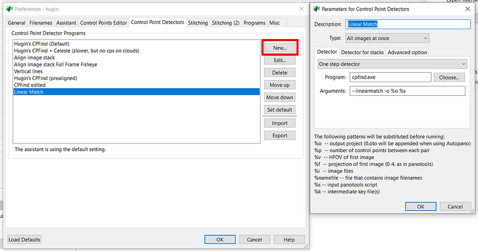
Name it Linear Match, and under the Detector tab, enter:
cpfind.exeUnder Arguments, enter:
--linearmatch -o %o %sAnd Linear Match should now show up in the Feature Matching section of the Photos tab. Pro tip: the matching distance can be modified by adding the argument
--linearmatchlen 2which would check image pairs 0-1, 0-2, 1-2, 1-3, 2-3, 2-4... (a different number can be substituted to adjust the matching distance).
After running CPFind with Linear Match, I then run CPFind (prealigned). After running these two detectors, I calculate the Geometric optimization and then Preview panorama (OpenGL). I can then find control points for a subset of images, depending on where Hugin is struggling.
In the Photos tab, you can select a subsample of images (I find that selecting < 40 images works best) and then run Feature Matching so that control points will only be generated for images within that subsample. Then, you can run another subsample, and so on and so forth, until all of the overlapping images have control points. The process may have to be repeated because certain combinations of neighbours will be missing. Another idea is to import a few images first, and then add images as you go.
Blending
Another issue with large images occurs during the stitching process. The stitching process consists of several stages:
Geometric optimization, which lines up the features/control points and estimates the positions of the images.
Stitching and photometric optimization, where the images are overlain and the exposures are normalized across all images.
Blending, where the boundaries between tiles are removed and smoothed so that features aren't duplicated at the boundaries.
In the blending stage, Hugin uses the Enblend tool, which is manageable for < 100 megapixels/images. But the Enblend tool has a computation time on the order of (𝑚 × 𝑛)² tiles because it incrementally blends tiles to an increasingly larger intermediate image. This computation time makes it impossible to handle blending larger images (one of my 450 megapixel mosaics had to be cancelled because it was blending indefinitely). The Multiblend tool solves this issue by effectively blending all of the images simultaneously, leading to a computation time on the order of 𝑚 × 𝑛.
To use Multiblend:
In Hugin, go to File > Preferences.
Under the Programs tab, find the Enblend section and check Use alternative Enblend program.
Click Choose... and locate where multiblend.exe is stored on your computer.

Summary
In this blog post, we showed that stitching images into mosaics can be done for free, using the open-source software Hugin. We also considered some of the complications and modifications to consider when stitching larger image sets (> 100 megapixels). So, what cool samples are you looking at under the microscope? Let me know in the comments below!
Hello! Thank you very much for your tutorial! It's the HELP I was looking for as I'm also working on microscopic images.
To answer your question: my cool samples are dental tissue 😁 Have a nice day and good luck with your PhD (if it is not yet finished) or or else congratulations!